What is BigQuery

BigQuery is Google’s platform to store and analyze large datasets. It is very fast and well integrated to other Google products such as cloud storage, and it’s free to use for up to 1TB of data analyzed each month, and up to 10GB of data stored. As any other database, it understands SQL and the online editor is a friendly place to learn and troubleshoot your queries. Big Query understands both Legacy and Standard SQL. Unfortunately, these languages are more different that you would expect, which makes things confusing. In this post I will use Standard SQL since Big Query is slowly migrating to only using this language in the future

To start using BigQuery, you need to have a gmail account and a Big Query-enabled project. If you don’t have this yet, please follow the steps in this quickstart guide quickstart guide and come back when done.

Global Fishing Watch’s data in BigQuery

Now that you have a BigQuery-enabled project, go the BigQuery’s UI page. You should see your project in the side bar, above the Public Datasets project. Click on the small arrow next to your project name, then switch to project -> display project, and enter “global-fishing-watch” (without the quotes) on the Project ID. Click OK, and you should then have a global-fishing-watch project in your side bar. This project contains, two datasets: "gfw_public_data" and "global_footprint_of_fisheries". We will work on the latter, which contains the public data released with the Science publication. This dataset contains the following four tables:

• fishing_effort: Daily Fishing Effort and Vessel Presence at 100th Degree Resolution by Flag State and Gear Type, 2012-2016
• fishing_effort_byvessel:Daily Fishing Effort at 10th Degree Resolution by MMSI, 2012-2016
• fishing_vessels: Characteristics of each vessel included in the effort data
• vessels: This table includes all vessels that were matched to a registry, were identified through manual review or web searchers, or were classified by the neural network.

Establishing a connection

The first step to use the data from R, is to set a connection with BigQuery. This is done using the DBI and bigrquery packages:

library(DBI)
library(bigrquery)

BQ_connection <-  dbConnect(bigquery(), 
                            project = 'global-fishing-watch',
                            dataset = "global_footprint_of_fisheries", 
                            billing = "ng-gfw", # your billing account name
                            use_legacy_sql = FALSE) # specify we are using Standard SQL

We then need to authenticate the connection. This can be done when running your first query such as listing the tables in your connection through the function dbListTable(). This will trigger a prompt in your R session asking if you want to cache your credentials. Allow access and return to RStudio.

DBI::dbListTables(BQ_connection)

## [1] "fishing_effort"          "fishing_effort_byvessel"
## [3] "fishing_vessels"         "vessels"

Now we are all set to start querying and analyzing Global Fishing Watch’s data. There are a couple of approaches to do this and whichever you use depends primarily on: 1) your experience with SQL, 2) how much you dislike SQL, and 3) how much you use R notebooks as opposed to classic R scripts. To illustrate these approches, I will walk through 3 simple analyses that exemplify the type of queries you may want to do:

1. Summarize the number of fishing vessels by flag state
2. Make a time series of fishing effort for China’s trawlers fleet
3. Make a map of fishing effort for a particular region of the ocean

The first example shows how to query data without writing a single SQL statement by leveraging the power of the dbplyr package. While very convenient, this approach has some limitations that I will mention below. The second and third examples use workflows that require you to write SQL, but give you more control and flexibility to do more interesting and complex queries. These, in my experience, are the best ways to unleash the full potential of Google Big Query and Global Fishing Watch’s data and I highly recommend you to explore them.

1. Summarize the number of vessels by flag state and gear type

This is possibly one the first and simplest queries to do. For this use case, we will use the dbplyr and bigrquery packages that allow us to avoid the need to write SQL. We just write the dplyr verbs and functions we all love, and the dbplyr package translates them into SQL in the back-end. The main advantages of this approach is that it’s very friendly and readable, and prevents us from the cognitive overhead of switching between programming languages. However, SQL is a very large language and dbplyr does not do everything; it focuses on SELECT statements which are often what we use the most.

The first step here is to connect to the table we want to query using the tbl() function:

library(tidyverse) #loads dplyr and friends

fishing_vessels <- dplyr::tbl(BQ_connection, 
                              "fishing_vessels") # connects to a table

However, notice that the variable created in your environment is not a dataframe or tibble but instead a list. This is because tbl() creates a reference to the table in the remote database but does not bring the actual data into memory. When you print it out, you’ll see it looks like a tibble but the class is tbl_sql.

fishing_vessels

## # Source:   table<fishing_vessels> [?? x 11]
## # Database: BigQueryConnection
##      mmsi flag  geartype length tonnage engine_power active_2012
##     <int> <chr> <chr>     <dbl>   <dbl>        <dbl> <lgl>      
##  1 6.03e8 AGO   trawlers   32.8    299.         734. FALSE      
##  2 6.03e8 AGO   trawlers   34.6    396.         865. FALSE      
##  3 6.03e8 AGO   trawlers   28.8    264.         652. FALSE      
##  4 6.03e8 AGO   trawlers   30.7    300.         704. FALSE      
##  5 6.03e8 AGO   trawlers   37.5    406.         851. FALSE      
##  6 6.03e8 AGO   trawlers   27.4    277.         749. FALSE      
##  7 6.03e8 AGO   trawlers   32.4    442.         889. FALSE      
##  8 6.03e8 AGO   trawlers   37.8    444.         887. FALSE      
##  9 6.03e8 AGO   trawlers   32.4    396.         812. FALSE      
## 10 6.04e8 AGO   purse_s…   36.8    292.        1182. TRUE       
## # ... with more rows, and 4 more variables: active_2013 <lgl>,
## #   active_2014 <lgl>, active_2015 <lgl>, active_2016 <lgl>

class(fishing_vessels)

## [1] "tbl_dbi"  "tbl_sql"  "tbl_lazy" "tbl"

The most important difference between a local dataframe and a remote dataframe of class tbl_sql is that in the latter your R code will run directly the database, not in memory. To do this efficiently, dplyr will be as lazy as possible by 1) not pulling data into R unless explicitly asked to, and 2) delaying the actual communication to the database until the last possible moment (i.e., after it collects all that you want to do).

Now, we can continue to use the dplyr verbs we are familiar with and summarize the table as we wish:

summary_by_country_and_gear <- fishing_vessels %>% 
  filter(active_2016) %>% 
  group_by(flag, geartype) %>% 
  summarize(n_vessels = n_distinct(mmsi),
            total_GT = sum(tonnage)) %>% 
  arrange(desc(n_vessels))

Again, the object created in our environment is not the dataframe we expected. In fact, the above code never touched the database, it only recorded the instructions to query the data. To pull the data into a local tibble we need to explicitly ask for it with the function collect().

summary_by_country_and_gear <- collect(summary_by_country_and_gear)

Now we have an actual dataframe with which we can make a simple summarizing plot:

top_20_flags <- summary_by_country_and_gear %>% 
  group_by(flag) %>% 
  summarize(n_vessels = sum(n_vessels)) %>% 
  top_n(20, n_vessels) %>% 
  pull(flag)

summary_by_country_and_gear %>% 
  filter(flag %in% top_20_flags) %>% 
  na.omit() %>% 
  ggplot(aes(x = forcats::fct_reorder(flag, n_vessels), y = n_vessels, fill = geartype))+
  geom_col()+
  coord_flip()+
  labs(x  = "")+
  hrbrthemes::theme_ipsum()+
  ggsci::scale_fill_startrek()

Chinese Trawlers are, by far, the largest fleet in the Global Fishing Watch Database.

This approach is straight forward and works perfectly for simple queries. However, I recommend you become proficient with SQL to make the most of the power of BigQuery and Global Fishing Watch data. This will help you troubleshoot when things don’t work as expected and it will make it easier to reach out to the Global Fishing Watch community for help. A couple of great resources to learn are: Learn SQL | Codecademy, and Learn SQL the Hard Way. Another way to start learning SQL is to use the function show_query() from dplyr, which will show you what your R code gets translated as in SQL, behind scenes.

fishing_vessels %>% 
  filter(active_2016) %>% 
  group_by(flag, geartype) %>% 
  summarize(n_vessels = n_distinct(mmsi),
            total_GT = sum(tonnage)) %>% 
  arrange(desc(n_vessels)) %>% 
  show_query()

## <SQL>
## SELECT `flag`, `geartype`, COUNT(DISTINCT `mmsi`) AS `n_vessels`, SUM(`tonnage`) AS `total_GT`
## FROM `fishing_vessels`
## WHERE (`active_2016`)
## GROUP BY `flag`, `geartype`
## ORDER BY `n_vessels` DESC

2. Make a time series of fishing effort for China’s trawlers fleet

fishing_vessels <- dplyr::tbl(BQ_connection, "fishing_vessels")
fishing_effort_byvessel <- dplyr::tbl(BQ_connection, "fishing_effort_byvessel")

ts_china_effort <- fishing_effort_byvessel %>% 
  inner_join(fishing_vessels %>% 
               filter(flag == "CHN", geartype == "trawlers"), by = "mmsi") %>% 
  group_by(date) %>% 
  summarize(fishing_hours = sum(fishing_hours, na.rm = T)) %>% 
  ungroup() %>% 
  arrange(date) %>% 
  collect()

head(ts_china_effort)

## # A tibble: 6 x 2
##   date       fishing_hours
##   <chr>              <dbl>
## 1 2012-01-06         11.0 
## 2 2012-01-07         20.6 
## 3 2012-01-08         10.7 
## 4 2012-01-09          7.53
## 5 2012-01-10          4.36
## 6 2012-01-11         17.4

# Define your variables
min_year <- 2012
gear <- "trawlers"
flag <- "CHN"

# Query to get effort by mmsi and date after 2012
all_effort_by_mmsi_query <- glue::glue_sql(
  '
  Select
  date,
  mmsi,
  fishing_hours
  FROM
  `global-fishing-watch.global_footprint_of_fisheries.fishing_effort_byvessel`
  WHERE   
  EXTRACT(YEAR FROM PARSE_DATE("%F",date)) > {min_year}
  ',
  .con = BQ_connection
  )

# Query to extract only chinese trawlers
chinese_vessels_sub_query <- glue::glue_sql(
  "
  Select
  mmsi
  FROM
  `global-fishing-watch.global_footprint_of_fisheries.fishing_vessels`
  WHERE flag = {flag}
  AND geartype = {gear}
  ",
  .con = BQ_connection
  )

full_sql <- glue::glue_sql(
  "
  SELECT
  date,
  sum(fishing_hours) AS fishing_hours
  FROM ({all_effort_by_mmsi_query}) AS a
  LEFT JOIN  ({chinese_vessels_sub_query}) AS b
  ON a.mmsi = b.mmsi
  GROUP BY date
  ORDER BY date
  DESC
  ",
  .con = BQ_connection
  )

full_sql

## <SQL> SELECT
## date,
## sum(fishing_hours) AS fishing_hours
## FROM (Select
## date,
## mmsi,
## fishing_hours
## FROM
## `global-fishing-watch.global_footprint_of_fisheries.fishing_effort_byvessel`
## WHERE   
## EXTRACT(YEAR FROM PARSE_DATE("%F",date)) > 2012) AS a
## LEFT JOIN  (Select
## mmsi
## FROM
## `global-fishing-watch.global_footprint_of_fisheries.fishing_vessels`
## WHERE flag = 'CHN'
## AND geartype = 'trawlers') AS b
## ON a.mmsi = b.mmsi
## GROUP BY date
## ORDER BY date
## DESC

china_trawlers_ts <- dbGetQuery(BQ_connection, 
                                full_sql)

moratoria_dates <- tibble(year = c(2013:2016)) %>% 
  mutate(start_date = lubridate::ymd(paste(year,"-06-01",sep = "")),
         end_date = lubridate::ymd(paste(year,"-08-01",sep = "")))

new_year_dates <- tibble(year = c(2013:2016),
                         start_date = c(lubridate::ymd("2013-02-07"),
                                        lubridate::ymd("2014-01-28"),
                                        lubridate::ymd("2015-02-16"),
                                        lubridate::ymd("2016-02-05")),
                         end_date = c(lubridate::ymd("2013-02-13"),
                                      lubridate::ymd("2014-02-3"),
                                      lubridate::ymd("2015-02-22"),
                                      lubridate::ymd("2016-02-11")))

ggplot() +
  geom_rect(data = moratoria_dates, 
            aes(xmin = start_date, 
                xmax = end_date,
                ymin = 0,
                ymax = Inf,
                fill = "navyblue"),
            alpha = 0.5, 
            show.legend = TRUE) +
  geom_rect(data = new_year_dates, 
            aes(xmin = start_date, 
                xmax = end_date,
                ymin = 0,
                ymax = Inf,
                fill = "dodgerblue"),
            alpha = 0.5,
            show.legend = TRUE) +
  geom_line(data = china_trawlers_ts %>% 
               mutate(date = lubridate::ymd(date)) %>% 
               filter(lubridate::year(date) > 2012),
           aes(x = date, y = fishing_hours), 
           size = 0.3)+
  theme_minimal() +
  theme(axis.ticks = element_line(size = 0.5),
        panel.grid.major = element_blank(), 
        panel.grid.minor = element_blank(),
        panel.background = element_blank(), 
        axis.line = element_line(colour = "black"),
        axis.text.y = element_text(size = 10),
        axis.text.x = element_text(size = 10),
        axis.title = element_text(size = 10),
        legend.text = element_text(size = 6),
        legend.justification = "center",
        legend.position = "bottom",
        plot.margin = margin(2,2,2,2)) + 
  scale_x_date(date_breaks = "1 year", 
               date_labels = "%Y ") +
  xlab("") +
  scale_y_continuous(expand = c(0, 0),
                     labels = scales::comma) +
  ylab("Fishing hours")+
  scale_fill_manual(values = c("orange", "dodgerblue"),
                    name = " ",
                    labels = c("Chinese New Year", "Moratoria")) +
  guides(colour = guide_legend(override.aes = list(alpha = .5)))

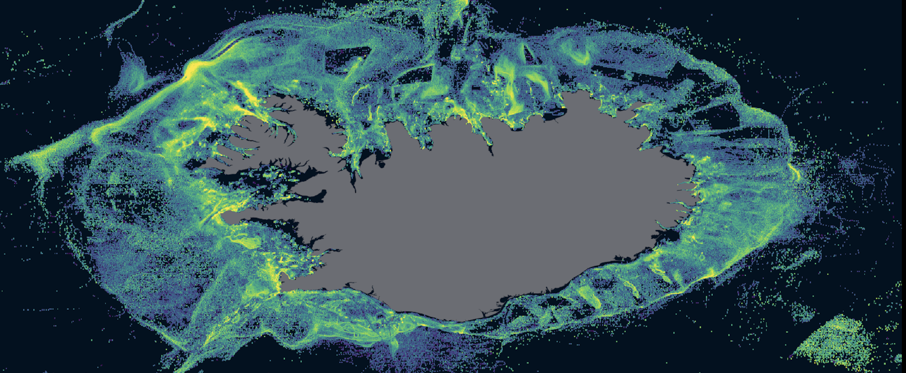
3. Make a map of fishing effort for a particular region of the ocean

A common use of Global Fishing Watch’s data is to make maps of fishing effort in an area of interest. I will show how you can do this and highlight another approach to query data from within R, using R Notebooks and chunks. For this, let’s make a map of fishing effort around the Azores Archipelago, Portugal.

If you are not familiar with R Notebooks, they are a type of code script that allows you to mix prose and code in a single document, with chunks of code that can be run independently and interactively. This is called literate programming, and makes analysis easier to reproduce. In fact, this tutorial is an R Notebook!. For more details on R Notebooks take a look at R Markdown: The Definitive Guide by Yihui Xie. One important advantage of R Notebooks is that chunks of code can use pretty much any programming language. This means that you could mix python, SQL, and R in a single, easy to read document! For our example we will use a SQL chunk to directly write an SQL query and get the data of fishing effort around the Azores.

First, lets get a map of the Azores to obtain the bounding of of our region of interest. To do this we can use the mregions package and a couple handy functions from the sf package.

# get the shapefile from mregions

azores_eez <- mregions::mr_shp(key = "MarineRegions:eez",
                 filter = "Portuguese Exclusive Economic Zone (Azores)",
                 maxFeatures = 200)

# transform the shapefile into an sf object
azores_eez <- azores_eez %>% 
  sf::st_as_sf()

# get the bounding box of the shapefile
azores_bbox <- sf::st_bbox(azores_eez)

# extend the bounding box 1 degree in every direction.
min_lon <- azores_bbox[["xmin"]] - 1 
max_lon <- azores_bbox[["xmax"]] + 1
min_lat <- azores_bbox[["ymin"]] - 1
max_lat <- azores_bbox[["ymax"]] + 1 

# define mapping resoluion in degrees
resolution <- 0.1

Now, we query the data. To do this with a sql chunk, we need to simply specify the language we are using (sql), the database connection (same as before), and the name we want to give to the variable that will contain the results of the query.

```{sql connection = BQ_connection, output.var = "binned_effort_around_Azores", echo = FALSE}
SELECT
  FLOOR(lat_bin/?resolution)*?resolution + 0.5*?resolution lat_bin_center,
  FLOOR(lon_bin/?resolution)*?resolution + 0.5*?resolution lon_bin_center,
  SUM(fishing_hours) fishing_hours
FROM (
  SELECT
    lat_bin/100 lat_bin,
    lon_bin/100 lon_bin,
    fishing_hours
  FROM
    `global-fishing-watch.global_footprint_of_fisheries.fishing_effort`
  WHERE
    _PARTITIONTIME >= '2016-01-01 00:00:00'
    AND _PARTITIONTIME < '2016-12-31 00:00:00')
  WHERE 
  lat_bin >= ?min_lat
  AND lat_bin <= ?max_lat
  AND lon_bin >= ?min_lon
  AND lon_bin <= ?max_lon
GROUP BY
  lat_bin_center,
  lon_bin_center
HAVING 
  fishing_hours > 0
```

OK, so what just happened here? First, we filtered the data for the year 2016 and converted the coordinates from 100th of a degree to degrees (See table schema in BigQuery). Then we filtered the coordinates so that they are inside our bounding box. To do this we add ? before the name of our locally defined variable and its value gets automagically added to the query. Lastly, we group and summarize the effort data with a resolution of 0.1º degrees and exclude anything with no fishing effort.

binned_effort_around_Azores %>% 
  filter(fishing_hours > 1) %>% 
  ungroup() %>% 
  ggplot()+
  geom_raster(aes(x = lon_bin_center, y = lat_bin_center, fill = fishing_hours))+
  viridis::scale_fill_viridis(name = "Fishing hours" ,
                              trans = "log",
                              breaks = scales::log_breaks(n = 10, base = 4))+
  geom_sf(data = azores_eez,
            fill = NA,
            col = "black",
            size = 1.4
            ) +
   hrbrthemes::theme_ipsum()+
  labs(title = "Fishing effort inside and around Azores",
       subtitle = "2017",
       y = "",
       x = "")+
    theme(axis.text.x = element_text(size = 10),
        axis.text.y = element_text(size = 10),
        plot.title = element_text(size = 14, hjust = 0),
        plot.subtitle = element_text(size = 14, hjust = 0),
        plot.margin = margin(10,0,0,0))

Closing remarks

Global Fishing Watch’s commitment to transparency and open source data, is rapidly changing the way we do research in fisheries science, and marine conservation. Powerful tools like Big Query and useful R packages (e.g., DBI, bigrquery, rmarkdown) are making these data accessible and easy to analyze, which will hopefully increase the rate it’s being used and the impact it can have. Have fun!